ID: GWAS-L03Type: Conceptual + ImplementationAudience: PublicTheme: Variant filtering, sample QC, and structure diagnostics
Why Genotype QC Matters
Association testing assumes:
Genotypes are measured reliably
Variants are polymorphic
Missingness is not systematic
Population structure is properly characterized
If these assumptions fail, false positives can arise before modeling even begins.
Genotype QC is not a preprocessing formality. It is statistical risk control.
Load Genotype Matrix
For demonstration, we use a simulated genotype matrix where:
Rows = samples
Columns = SNPs
Values = 0, 1, 2 (allele dosage)
<- read.csv ("data/demo-genotypes.csv" , row.names = 1 )dim (geno)
           rs1 rs2 rs3 rs4 rs5 rs6
sample-001   0   0   0   0   1   2
sample-002   0   0   0   1   0   1
sample-003   0   0   0   1   0   1
sample-004   1   0   0   0   0   1
sample-005   0   0   0   0   0   0
Missingness Per SNP
Variants with excessive missing data can bias association tests.
<- colMeans (is.na (geno))summary (snp_missing)
   Min. 1st Qu.  Median    Mean 3rd Qu.    Max.
 0.0000  0.0250  0.0350  0.0379  0.0500  0.1350
A typical threshold in practice might be 2–5% missingness. For this demo, we filter SNPs with >5% missingness.
<- geno[, snp_missing <= 0.05 ]dim (geno_filtered)
Minor Allele Frequency (MAF)
Very rare variants can:
Inflate variance estimates
Produce unstable effect sizes
Generate extreme p-values due to sparse counts
Compute allele frequency and MAF.
<- colMeans (geno_filtered, na.rm = TRUE ) / 2 <- pmin (allele_freq, 1 - allele_freq)summary (maf)
   Min. 1st Qu.  Median    Mean 3rd Qu.    Max.
 0.0285  0.1601  0.2784  0.2764  0.3952  0.5000
Filter SNPs with MAF < 0.05.
<- geno_filtered[, maf >= 0.05 ]dim (geno_filtered)
Interpretation:
Removing very rare variants increases model stability in small datasets. In large biobank-scale GWAS, rare variant strategies differ and require specialized modeling.
Sample-Level Missingness
Samples with excessive missing genotypes can distort association signals.
<- rowMeans (is.na (geno_filtered))summary (sample_missing)
    Min.  1st Qu.   Median     Mean  3rd Qu.     Max.
0.003207 0.008980 0.023412 0.029548 0.042335 0.124439
Filter samples with >5% missingness.
<- sample_missing <= 0.05 <- geno_filtered[keep_samples, ]dim (geno_filtered)
Principal Component Analysis (PCA)
Population structure is estimated from genotype variation.
Before PCA, we use simple mean imputation to avoid dropping large parts of the genotype matrix due to missingness. This is a pragmatic step for structure estimation, not a claim about true genotypes.
<- as.matrix (geno_filtered)for (j in seq_len (ncol (geno_mat))){<- is.na (geno_mat[, j])if (any (idx)){<- mean (geno_mat[, j], na.rm = TRUE )<- mustopifnot (! anyNA (geno_mat))
For teaching stability and speed, we run PCA on a subset of SNPs.
set.seed (1 )<- min (1000 , ncol (geno_mat))<- sample (seq_len (ncol (geno_mat)), size = m_use)<- geno_mat[, keep_snps, drop = FALSE ]dim (geno_mat_pca)
Scaling can fail if any SNP has zero variance (all values identical). We drop such SNPs before PCA.
<- apply (geno_mat_pca, 2 , stats:: sd)<- is.finite (sds) & sds > 0 <- geno_mat_pca[, keep_var, drop = FALSE ]dim (geno_mat_pca)
<- scale (geno_mat_pca)stopifnot (! anyNA (geno_scaled))stopifnot (all (is.finite (geno_scaled)))<- prcomp (geno_scaled, center = FALSE , scale. = FALSE )summary (pca)$ importance[2 , 1 : 5 ]
    PC1     PC2     PC3     PC4     PC5
0.01193 0.01147 0.01133 0.01127 0.01114
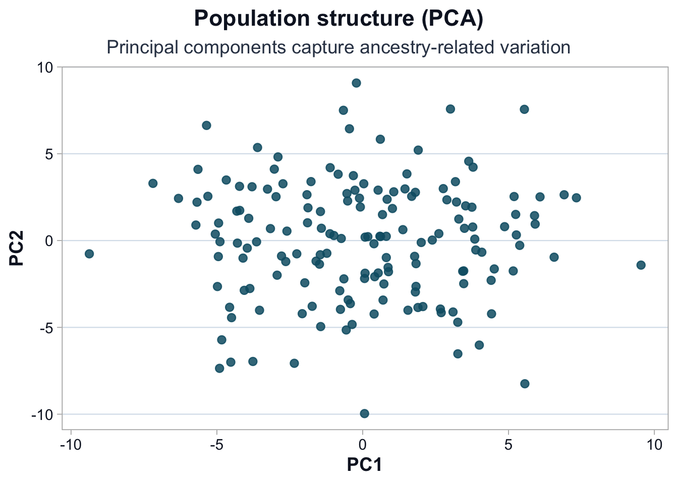
Visualize PC1 vs PC2
source ("scripts/R/cdi-plot-theme.R" )library (ggplot2)<- data.frame (PC1 = pca$ x[, 1 ],PC2 = pca$ x[, 2 ]<- cdi_palette ()ggplot (pca_df, ggplot2:: aes (x = PC1, y = PC2)) + :: geom_point (color = pal$ teal,alpha = 0.85 ,size = 2.4 + :: labs (title = "Population structure (PCA)" ,subtitle = "Principal components capture ancestry-related variation" ,x = "PC1" ,y = "PC2" + cdi_theme ()
Interpretation
Principal components summarize correlated genotype variation.
Clusters or gradients suggest:
Ancestry differences
Batch effects
Subpopulation structure
Ignoring population structure can produce systematic association inflation.
What QC Achieved
After QC, we have:
Removed poorly genotyped variants
Excluded unstable rare variants
Filtered low-quality samples
Estimated ancestry structure
Association testing now operates on a more stable genotype matrix.