Lesson 6: From Association to Biological Claims

• ID: GWAS-L06
• Type: Interpretation Discipline
• Audience: Public
• Theme: Calibration, plausibility, and responsible reporting

Why This Lesson Exists

A statistically significant association is not automatically a biological discovery.

GWAS identifies statistical relationships between genotype and phenotype. It does not automatically establish causality, mechanism, or clinical relevance.

This lesson focuses on disciplined interpretation.

---

Recompute Results (Self-Contained)

source("scripts/R/cdi-plot-theme.R")
library(ggplot2)

pheno <- read.csv("data/demo-phenotype.csv", stringsAsFactors = FALSE)
covar <- read.csv("data/demo-covariates.csv", stringsAsFactors = FALSE)
geno  <- read.csv("data/demo-genotypes.csv", row.names = 1)

df <- merge(pheno, covar, by = "sample_id")

common_ids <- intersect(df$sample_id, rownames(geno))
df   <- df[match(common_ids, df$sample_id), ]
geno <- geno[common_ids, , drop = FALSE]

test_snp_lm <- function(x, df){
  if (any(is.na(x))){
    x[is.na(x)] <- mean(x, na.rm = TRUE)
  }
  fit <- lm(trait ~ x + age + sex + PC1 + PC2, data = df)
  co <- summary(fit)$coefficients
  c(
    beta = unname(co["x", "Estimate"]),
    se   = unname(co["x", "Std. Error"]),
    p    = unname(co["x", "Pr(>|t|)"])
  )
}

res <- t(apply(geno, 2, test_snp_lm, df = df))
res <- as.data.frame(res)
res$snp <- rownames(res)
res$logp <- -log10(res$p)

alpha_nominal <- 0.05
res$is_sig <- res$p < alpha_nominal

res <- res[order(res$p), ]
head(res, 5)

            beta        se            p   snp     logp is_sig
rs153  0.6862770 0.1030083 2.714428e-10 rs153 9.566322   TRUE
rs754 -0.7736402 0.1873225 5.388030e-05 rs754 4.268570   TRUE
rs229 -0.4507871 0.1184809 1.901932e-04 rs229 3.720805   TRUE
rs424  0.3982625 0.1161028 7.366738e-04 rs424 3.132725   TRUE
rs593  0.3478399 0.1066971 1.315523e-03 rs593 2.880901   TRUE

---

Effect Size Distribution

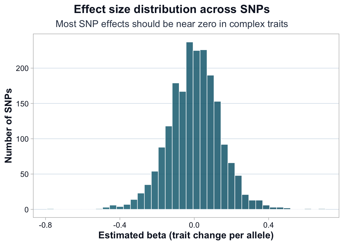
ggplot(res, aes(x = beta)) +
  cdi_geom_histogram(bins = 40, colored = TRUE) +
  cdi_scale_histogram_fill() +
  labs(
    title = "Effect size distribution across SNPs",
    subtitle = "Most SNP effects should be near zero in complex traits",
    x = "Estimated beta (trait change per allele)",
    y = "Number of SNPs"
  ) +
  cdi_theme()

Interpretation

In complex traits, most variants have small effects. A symmetric distribution centered near zero is expected under polygenicity. Large-magnitude effects should be treated with caution and verified carefully.

---

Volcano-Style Calibration Plot

pal <- cdi_palette()

plot_df <- res
plot_df$sig_label <- ifelse(plot_df$is_sig,
                            "Nominally significant",
                            "Not significant")

ggplot(plot_df, aes(x = beta, y = logp)) +
  geom_point(aes(color = sig_label),
             alpha = 0.8,
             size = 1.8) +
  geom_vline(xintercept = 0,
             linewidth = 0.6,
             color = pal$muted) +
  geom_hline(yintercept = -log10(alpha_nominal),
             linetype = "dashed",
             linewidth = 0.6,
             color = pal$highlight) +
  scale_color_manual(values = c(
    "Not significant" = pal$teal_light,
    "Nominally significant" = pal$highlight
  )) +
  labs(
    title = "Effect size vs statistical evidence",
    subtitle = "Vertical line: no effect. Horizontal line: nominal threshold.",
    x = "Estimated beta",
    y = "-log10(p-value)",
    color = ""
  ) +
  cdi_theme()

Interpretation

The characteristic “V” shape is typical in GWAS.

• Points near beta = 0 show little evidence.
• Stronger effects with stable estimates rise above the threshold.
• Large betas with weak evidence often indicate instability or sparse genotype counts.

Significant points are candidates — not conclusions.

---

Sensitivity to Population Structure

top_snp <- res$snp[1]
x <- geno[, top_snp]

if (any(is.na(x))){
  x[is.na(x)] <- mean(x, na.rm = TRUE)
}

fit_adjusted   <- lm(trait ~ x + age + sex + PC1 + PC2, data = df)
fit_unadjusted <- lm(trait ~ x + age + sex, data = df)

adj   <- coef(summary(fit_adjusted))["x", ]
unadj <- coef(summary(fit_unadjusted))["x", ]

adj

    Estimate   Std. Error      t value     Pr(>|t|) 
6.862770e-01 1.030083e-01 6.662345e+00 2.714428e-10 

unadj

    Estimate   Std. Error      t value     Pr(>|t|) 
6.539695e-01 1.056920e-01 6.187505e+00 3.500449e-09 

Interpretation

If adjustment causes large shifts in effect magnitude or direction, the association may reflect ancestry structure rather than locus-specific biology.

Robust signals remain directionally consistent after adjustment.

---

Interpretation Hierarchy

Responsible GWAS interpretation follows layers:

1. Statistical evidence
   
2. Calibration and inflation diagnostics
   
3. Robustness to covariate adjustment
   
4. Replication
   
5. Biological plausibility
   
6. Functional validation

Skipping layers increases the risk of overstatement.

---

What This Free Track Achieved

You now understand:

• Study design logic
  
• Phenotype calibration
  
• Genotype QC
  
• Population structure control
  
• Per-SNP modeling
  
• Diagnostic calibration
  
• Interpretation discipline

The goal was not to produce hits.

The goal was to produce defensible reasoning.