Lesson 4 Quality Control Decisions
4.1 Why quality control is central to GWAS
Quality control (QC) is the foundation of a reliable GWAS.
QC decisions determine which samples and variants are included in the analysis.
Poor QC can introduce bias, inflate false positives, or reduce power in ways that are difficult to detect later.
QC is not a single step.
It is a sequence of decisions that shape the dataset used for association testing.
4.2 QC as a decision system
It is useful to think of QC as a system of filters rather than a checklist.
Each filter answers a question such as:
- Is this sample reliable?
- Is this variant measured with sufficient confidence?
- Does this data point behave consistently with expectations?
The goal is not to maximize sample size at all costs.
The goal is to retain data that support valid statistical inference.
4.3 Sample level quality control
Sample level QC focuses on identifying individuals whose data may compromise the analysis.
Common sample level checks include:
- missing genotype rate per individual
- sex consistency checks
- heterozygosity outliers
- duplicated or related samples
- ancestry outliers
Samples failing these checks may reflect technical problems, data mix ups, or population structure issues.
4.4 Variant level quality control
Variant level QC focuses on the reliability and informativeness of individual genetic variants.
Typical variant level checks include:
- call rate or missingness per variant
- minor allele frequency thresholds
- deviations from Hardy Weinberg equilibrium
- strand or allele inconsistencies
Variants failing these criteria may introduce noise or systematic bias into association tests.
4.5 Order of QC steps matters
QC steps are not independent.
For example:
- removing low quality samples can change variant level metrics
- excluding rare variants affects downstream power calculations
- ancestry related filtering influences Hardy Weinberg expectations
For this reason, QC is often performed iteratively rather than in a single pass.
4.6 Thresholds are context dependent
There is no universal set of QC thresholds that applies to all studies.
Threshold choices depend on:
- study design
- genotyping platform
- sample size
- population characteristics
- downstream analysis goals
QC thresholds should be justified and documented rather than copied blindly from other studies.
4.7 Inspecting QC signals in the demo dataset
To make QC ideas concrete, we use the CDI GWAS demo dataset introduced earlier.
In this foundations lesson, the goal is to inspect QC signals, not to apply a full QC pipeline.
We will:
- compute missingness per sample and per variant
- flag potential issues using example thresholds
- summarize what would happen if filters were applied
We will not permanently modify the dataset files.
from pathlib import Path
import pandas as pd

# Update this path if you store the dataset elsewhere
DATA_DIR = Path("data/gwas-demo-dataset")

phenotypes_path = DATA_DIR / "phenotypes.csv"
genotypes_path = DATA_DIR / "genotypes.csv"
variants_path = DATA_DIR / "variants.csv"

phenotypes = pd.read_csv(phenotypes_path)
genotypes = pd.read_csv(genotypes_path)
variants = pd.read_csv(variants_path)

phenotypes.head(), genotypes.iloc[:5, :6], variants.head()
( sample_id trait_binary trait_quant age sex pc1 pc2 pc3 \
0 S0001 1 -0.0108 43 F 1.6018 -1.0624 -0.8633
1 S0002 1 2.0082 56 M -0.2394 -0.5294 -0.1475
2 S0003 1 -0.7331 55 M -1.0235 -0.8769 -0.1525
3 S0004 1 -0.9815 44 F 0.1793 -0.0943 0.3834
4 S0005 0 1.5433 66 F 0.2200 -1.7577 0.9998
batch
0 site-b
1 site-a
2 site-b
3 site-b
4 site-c ,
sample_id rs100002 rs100005 rs100031 rs100018 rs100021
0 S0001 0.0 1.0 0.0 0.0 1.0
1 S0002 1.0 0.0 NaN 1.0 0.0
2 S0003 1.0 0.0 0.0 0.0 1.0
3 S0004 0.0 0.0 0.0 0.0 1.0
4 S0005 0.0 0.0 0.0 1.0 1.0,
snp_id chr pos ref alt maf
0 rs100002 1 6891850 A C 0.1962
1 rs100005 1 47496996 G A 0.0571
2 rs100031 1 156142503 G T 0.2254
3 rs100018 2 106591486 G A 0.2618
4 rs100021 2 131748289 G T 0.3114)4.7.1 Basic alignment checks
A minimal alignment check confirms that:
sample_idexists in both tables- sample identifiers are unique
- the overlap between genotype and phenotype samples is as expected
# Basic alignment checks
assert "sample_id" in phenotypes.columns
assert "sample_id" in genotypes.columns

n_pheno = phenotypes["sample_id"].nunique()
n_geno = genotypes["sample_id"].nunique()

overlap = set(phenotypes["sample_id"]).intersection(set(genotypes["sample_id"]))

summary = pd.DataFrame(
    {
        "table": ["phenotypes", "genotypes", "overlap"],
        "n_unique_samples": [n_pheno, n_geno, len(overlap)],
    }
)

summary| table | n_unique_samples | |
|---|---|---|
| 0 | phenotypes | 120 |
| 1 | genotypes | 120 |
| 2 | overlap | 120 |
4.7.2 Missingness per sample and per variant
Missingness is one of the first QC signals to inspect.
We compute:
- sample missingness as the fraction of missing genotype calls per individual
- variant missingness as the fraction of missing calls per variant
import numpy as np

geno_matrix = genotypes.drop(columns=["sample_id"])

sample_missing_rate = geno_matrix.isna().mean(axis=1)
variant_missing_rate = geno_matrix.isna().mean(axis=0)

sample_missing_rate.describe(), variant_missing_rate.describe()
(count 120.000000
mean 0.033542
std 0.028715
min 0.000000
25% 0.018750
50% 0.025000
75% 0.050000
max 0.125000
dtype: float64,
count 40.000000
mean 0.033542
std 0.016719
min 0.008333
25% 0.016667
50% 0.033333
75% 0.043750
max 0.075000
dtype: float64)4.7.3 Visualizing missingness
Plots are helpful for spotting outliers and long tails.
The goal here is to understand the distribution, not to enforce a single rule.
import matplotlib.pyplot as plt

plt.figure()
plt.hist(sample_missing_rate, bins=20)
plt.xlabel("Sample missingness rate")
plt.ylabel("Number of samples")
show_and_save_mpl()

plt.figure()
plt.hist(variant_missing_rate, bins=20)
plt.xlabel("Variant missingness rate")
plt.ylabel("Number of variants")
show_and_save_mpl()
Saved PNG → figures/04_001.png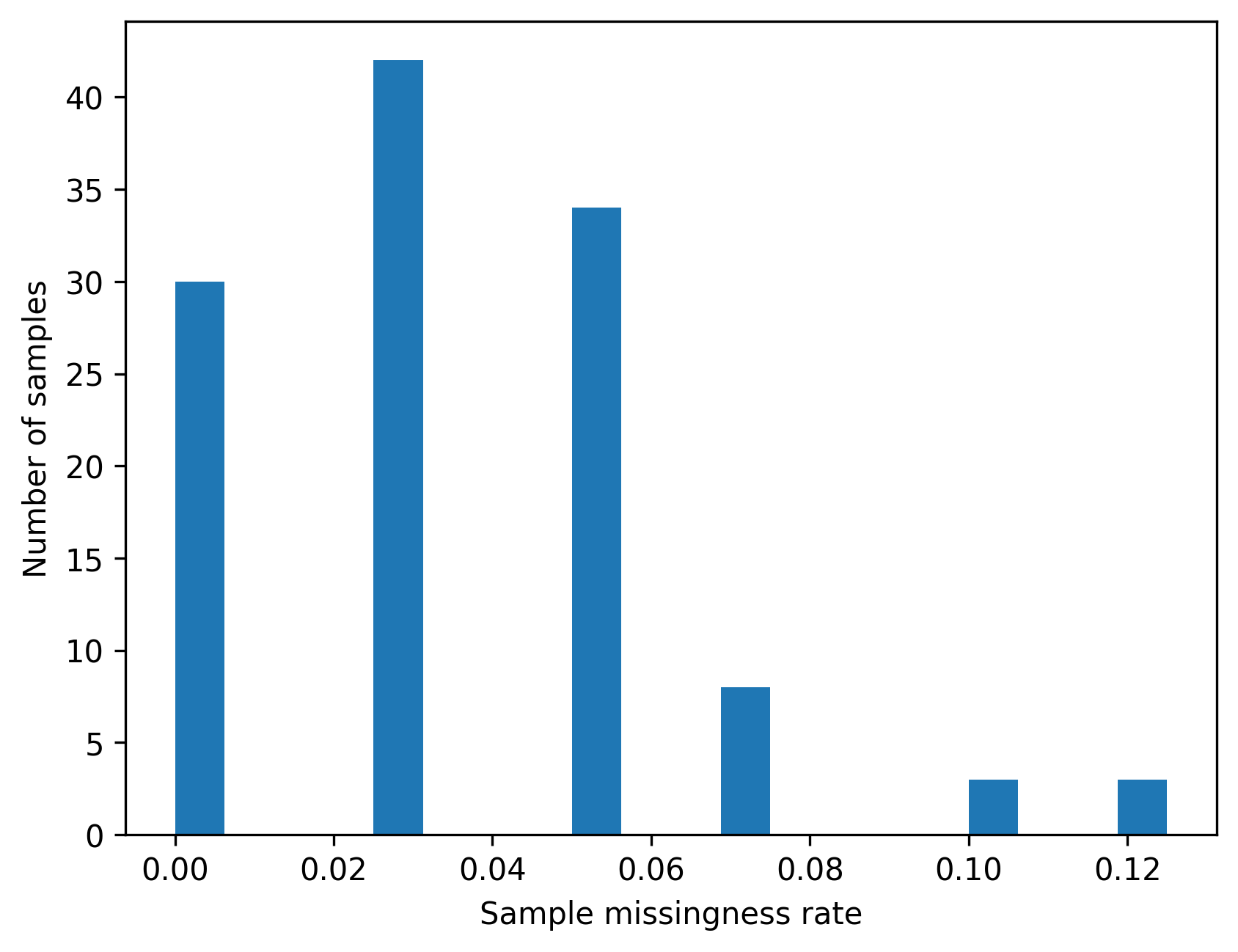
Saved PNG → figures/04_002.png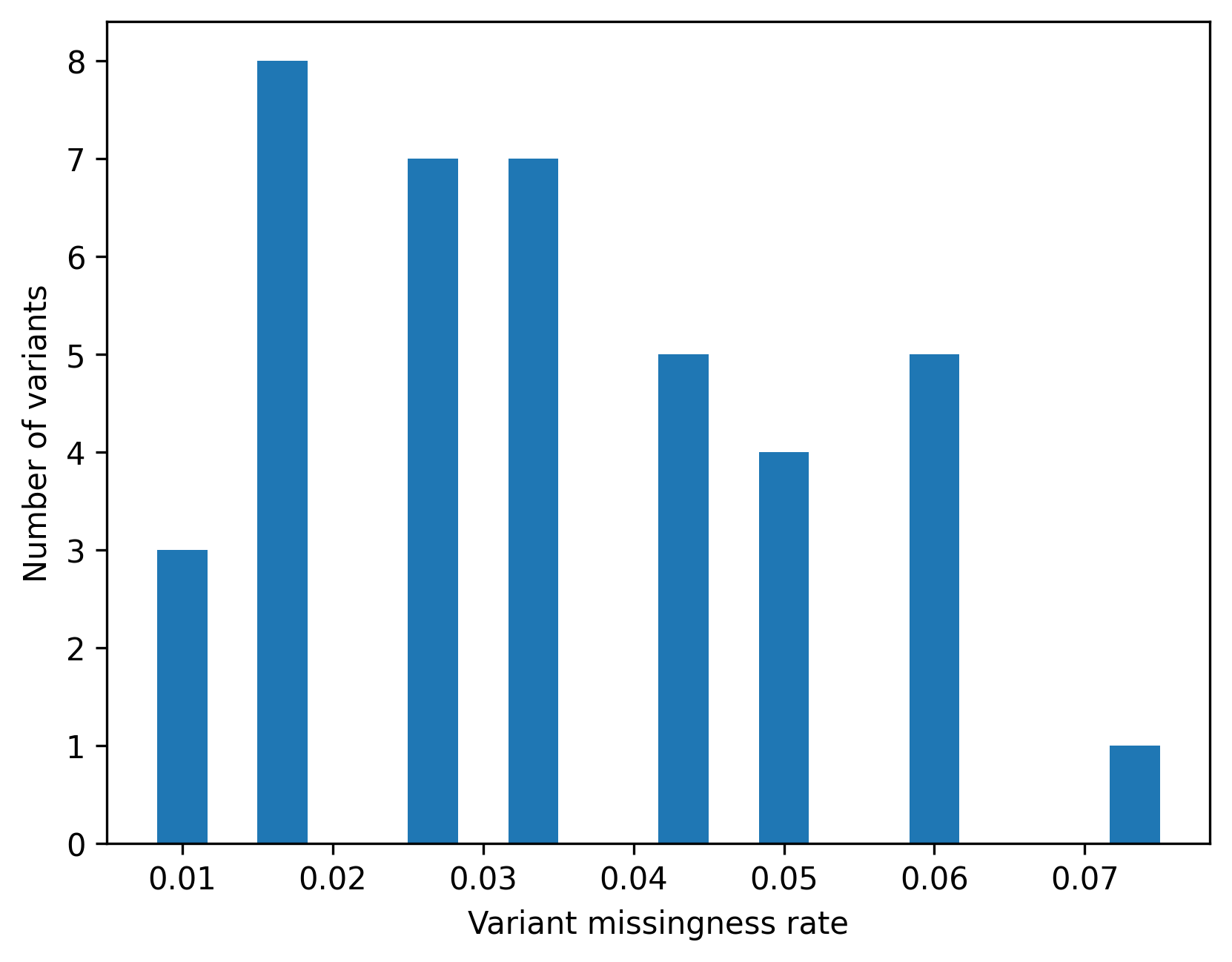
4.7.4 Example flags using illustrative thresholds
Thresholds are context dependent.
For teaching purposes, we flag samples or variants above an example missingness threshold.
These flags help you reason about the consequences of filtering.
# Example thresholds for illustration only
sample_missing_threshold = 0.05
variant_missing_threshold = 0.05

flag_sample_high_missing = sample_missing_rate > sample_missing_threshold
flag_variant_high_missing = variant_missing_rate > variant_missing_threshold

flag_summary = pd.DataFrame(
    {
        "item": ["samples", "variants"],
        "threshold": [sample_missing_threshold, variant_missing_threshold],
        "n_flagged": [int(flag_sample_high_missing.sum()), int(flag_variant_high_missing.sum())],
        "n_total": [int(len(flag_sample_high_missing)), int(len(flag_variant_high_missing))],
    }
)

flag_summary| item | threshold | n_flagged | n_total | |
|---|---|---|---|---|
| 0 | samples | 0.05 | 14 | 120 |
| 1 | variants | 0.05 | 6 | 40 |
4.8 QC and reproducibility
QC decisions must be reproducible.
This means:
- recording thresholds and filters used
- keeping track of sample and variant counts at each step
- saving intermediate datasets when appropriate
Clear QC documentation makes analyses easier to review, reproduce, and extend.
4.9 Key takeaways
- QC is a core component of GWAS, not a technical detail
- Both samples and variants require careful filtering
- QC decisions influence downstream results
- Thresholds should be study specific and justified
- Reproducible QC practices improve scientific reliability
Continue to → Lesson 05: Population Structure and Relatedness