Lesson 5 Population Structure and Relatedness
5.1 Why population structure matters in GWAS
GWAS assumes that genetic variants are tested in a population where individuals are comparable aside from the trait of interest.
In practice, study samples often include individuals from different ancestral backgrounds or with varying degrees of relatedness.
If population structure is not accounted for, genetic differences that reflect ancestry rather than biology can appear as false associations.
5.2 Population stratification
Population stratification refers to systematic differences in allele frequencies between subgroups of individuals.
These differences can arise from:
- ancestral history
- geographic separation
- migration and admixture
When stratification aligns with trait differences, it can confound association results.
5.4 Inspecting population structure in the demo dataset
To ground these ideas, we inspect population structure signals in the CDI GWAS demo dataset.
At this stage, the goal is to:
- understand what structure summaries look like
- learn how they are interpreted
- avoid premature filtering or modeling
We do not perform a full ancestry inference pipeline in this lesson.
from pathlib import Path
import pandas as pd

DATA_DIR = Path("data/gwas-demo-dataset")

phenotypes = pd.read_csv(DATA_DIR / "phenotypes.csv")
variants = pd.read_csv(DATA_DIR / "variants.csv")

phenotypes.head(), variants.head()
( sample_id trait_binary trait_quant age sex pc1 pc2 pc3 \
0 S0001 1 -0.0108 43 F 1.6018 -1.0624 -0.8633
1 S0002 1 2.0082 56 M -0.2394 -0.5294 -0.1475
2 S0003 1 -0.7331 55 M -1.0235 -0.8769 -0.1525
3 S0004 1 -0.9815 44 F 0.1793 -0.0943 0.3834
4 S0005 0 1.5433 66 F 0.2200 -1.7577 0.9998
batch
0 site-b
1 site-a
2 site-b
3 site-b
4 site-c ,
snp_id chr pos ref alt maf
0 rs100002 1 6891850 A C 0.1962
1 rs100005 1 47496996 G A 0.0571
2 rs100031 1 156142503 G T 0.2254
3 rs100018 2 106591486 G A 0.2618
4 rs100021 2 131748289 G T 0.3114)5.5 Ancestry components as summaries
In practice, population structure is often summarized using ancestry components.
These components:
- capture major axes of genetic variation
- reflect ancestry gradients or clusters
- can be used as covariates in association models
In the demo dataset, ancestry components are already provided as pc1, pc2, and pc3.
| pc1 | pc2 | pc3 | |
|---|---|---|---|
| count | 120.000000 | 120.000000 | 120.000000 |
| mean | -0.008994 | 0.061467 | -0.041772 |
| std | 1.011939 | 1.029519 | 0.990252 |
| min | -2.147300 | -2.566700 | -2.333600 |
| 25% | -0.750050 | -0.575950 | -0.714425 |
| 50% | -0.129700 | 0.112300 | -0.007250 |
| 75% | 0.562375 | 0.735825 | 0.570375 |
| max | 2.913900 | 2.905100 | 2.327700 |
5.6 Visualizing ancestry components
Plots of ancestry components help reveal:
- clusters of samples
- continuous gradients
- potential outliers
The goal is interpretation, not classification.
import matplotlib.pyplot as plt

plt.figure()
plt.scatter(phenotypes["pc1"], phenotypes["pc2"])
plt.xlabel("PC1")
plt.ylabel("PC2")
show_and_save_mpl()

plt.figure()
plt.scatter(phenotypes["pc1"], phenotypes["pc3"])
plt.xlabel("PC1")
plt.ylabel("PC3")
show_and_save_mpl()
Saved PNG → figures/05_001.png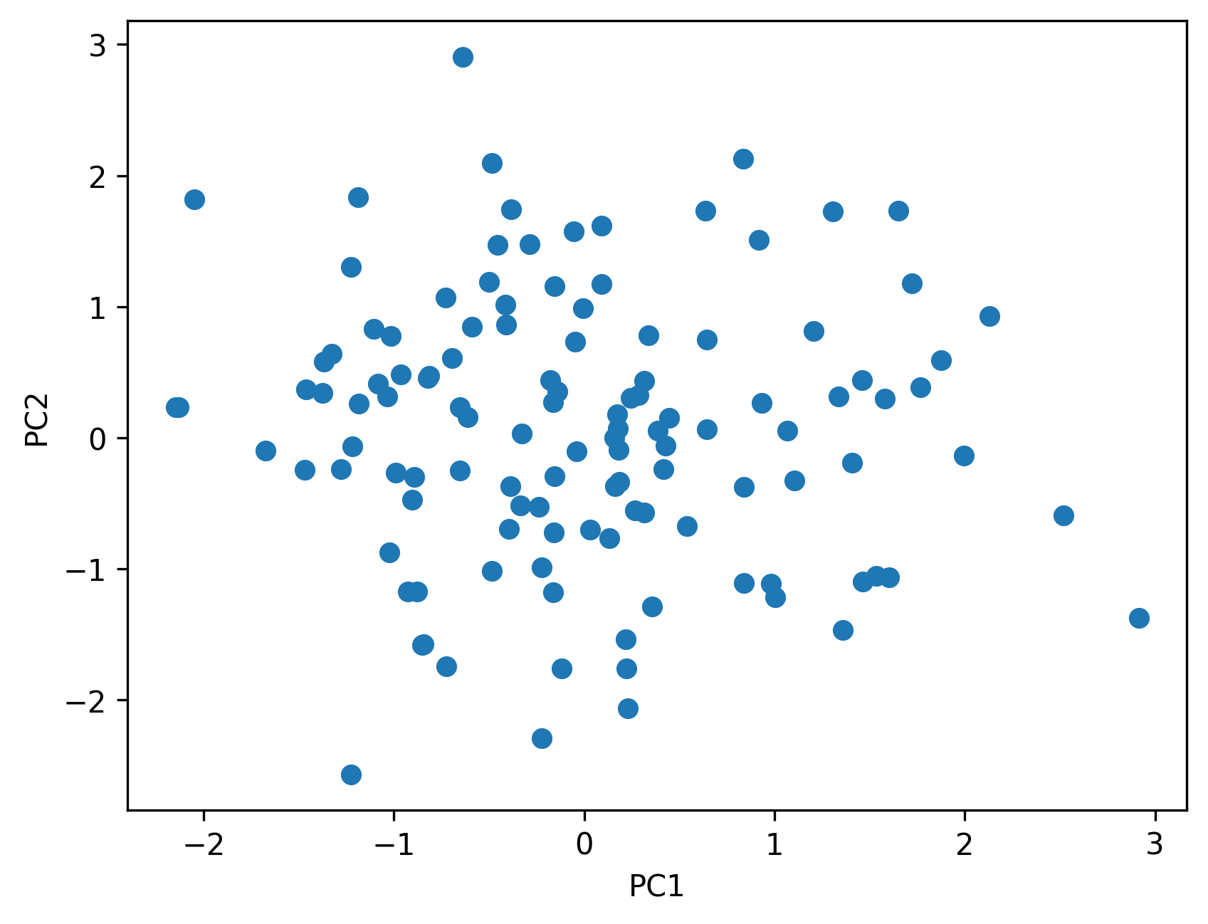
Saved PNG → figures/05_002.png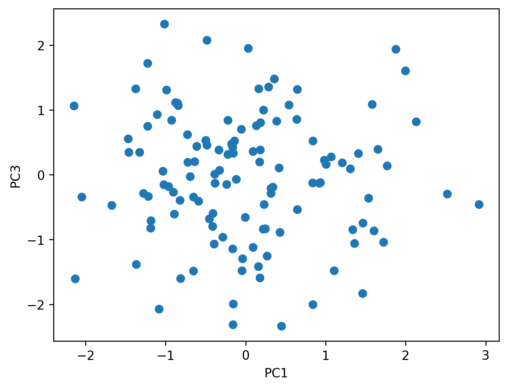
5.7 Structure as covariates
Rather than excluding individuals, GWAS commonly adjusts for structure.
This is done by:
- including ancestry components as covariates
- fitting models that account for relatedness directly
Adjustment helps control confounding while retaining sample size.
5.8 Structure versus signal
Not all population structure should be removed.
Some genetic signals may reflect true biological differences linked to ancestry.
The challenge is to distinguish:
- confounding structure
- meaningful genetic variation
This distinction requires careful interpretation and domain knowledge.
5.9 Key takeaways
- Population structure can confound GWAS results
- Relatedness violates independence assumptions
- Ancestry components summarize genetic structure
- Adjustment is often preferable to exclusion
- Interpretation requires care and context
Continue to → Lesson 06: Association Testing Models