Lesson 6 Association Testing Models
6.1 What we test in GWAS
In GWAS, we test whether genotype variation at a variant is associated with a phenotype.
In practice, we fit models that relate:
- outcome: quantitative trait or case-control status
- predictor: genotype (0, 1, 2 for additive coding)
- covariates: age, sex, and ancestry principal components
In this lesson, we:
- build a small analysis table from the demo dataset
- fit a baseline association model for one SNP
- run a small multi-SNP scan
- generate a QQ plot as a diagnostic summary
6.2 Load the demo dataset
import pandas as pd
import numpy as np

genotypes = pd.read_csv("data/gwas-demo-dataset/genotypes.csv")
phenotypes = pd.read_csv("data/gwas-demo-dataset/phenotypes.csv")

print("genotypes:", genotypes.shape)
print("phenotypes:", phenotypes.shape)
print("genotype columns (first 10):", list(genotypes.columns[:10]))
print("phenotype columns:", list(phenotypes.columns))
genotypes: (120, 41)
phenotypes: (120, 9)
genotype columns (first 10): ['sample_id', 'rs100002', 'rs100005', 'rs100031', 'rs100018', 'rs100021', 'rs100032', 'rs100035', 'rs100003', 'rs100037']
phenotype columns: ['sample_id', 'trait_binary', 'trait_quant', 'age', 'sex', 'pc1', 'pc2', 'pc3', 'batch']6.3 Merge phenotypes and genotypes
We merge on sample_id and prepare covariates.
If sex is encoded as F/M, we convert to 0/1.
import statsmodels.api as sm

df = phenotypes.merge(genotypes, on="sample_id", how="inner")

if "sex" in df.columns:
    df["sex"] = df["sex"].map({"F": 0, "M": 1})

candidate_covars = ["age", "sex", "pc1", "pc2", "pc3"]
covars = [c for c in candidate_covars if c in df.columns]

trait_col = "trait_quant"
if trait_col not in df.columns:
    raise KeyError(f"Expected phenotype column '{trait_col}' not found. Columns: {list(df.columns)}")

snp_cols = [c for c in genotypes.columns if c != "sample_id"]

print("Covariates used:", covars)
print("Number of SNP columns:", len(snp_cols))
print(df[[trait_col] + covars + snp_cols[:3]].head())
Covariates used: ['age', 'sex', 'pc1', 'pc2', 'pc3']
Number of SNP columns: 40
trait_quant age sex pc1 pc2 pc3 rs100002 rs100005 rs100031
0 -0.0108 43 0 1.6018 -1.0624 -0.8633 0.0 1.0 0.0
1 2.0082 56 1 -0.2394 -0.5294 -0.1475 1.0 0.0 NaN
2 -0.7331 55 1 -1.0235 -0.8769 -0.1525 1.0 0.0 0.0
3 -0.9815 44 0 0.1793 -0.0943 0.3834 0.0 0.0 0.0
4 1.5433 66 0 0.2200 -1.7577 0.9998 0.0 0.0 0.06.4 Baseline association model for one SNP
We demonstrate a single-variant association test using linear regression:
trait_quant ~ genotype + covariates
snp_demo = snp_cols[0]

X_cols = [snp_demo] + covars
X = df[X_cols].astype(float)
X = sm.add_constant(X)
y = df[trait_col].astype(float)

lin_model = sm.OLS(y, X, missing="drop").fit()

print("Demo SNP:", snp_demo)
print(lin_model.summary())
Demo SNP: rs100002
OLS Regression Results
==============================================================================
Dep. Variable: trait_quant R-squared: 0.373
Model: OLS Adj. R-squared: 0.339
Method: Least Squares F-statistic: 10.99
Date: Thu, 29 Jan 2026 Prob (F-statistic): 1.39e-09
Time: 01:22:33 Log-Likelihood: -140.55
No. Observations: 118 AIC: 295.1
Df Residuals: 111 BIC: 314.5
Df Model: 6
Covariance Type: nonrobust
==============================================================================
coef std err t P>|t| [0.025 0.975]
------------------------------------------------------------------------------
const -1.4663 0.247 -5.936 0.000 -1.956 -0.977
rs100002 0.2355 0.152 1.554 0.123 -0.065 0.536
age 0.0292 0.005 5.700 0.000 0.019 0.039
sex 0.1026 0.154 0.665 0.507 -0.203 0.408
pc1 0.3238 0.076 4.284 0.000 0.174 0.474
pc2 -0.1157 0.074 -1.565 0.120 -0.262 0.031
pc3 0.0089 0.078 0.113 0.910 -0.147 0.164
==============================================================================
Omnibus: 0.088 Durbin-Watson: 1.874
Prob(Omnibus): 0.957 Jarque-Bera (JB): 0.237
Skew: -0.040 Prob(JB): 0.888
Kurtosis: 2.795 Cond. No. 161.
==============================================================================
Notes:
[1] Standard Errors assume that the covariance matrix of the errors is correctly specified.6.5 Minimal association summary
assoc_summary = pd.DataFrame({
    "snp": [snp_demo],
    "beta": [float(lin_model.params.get(snp_demo, np.nan))],
    "se": [float(lin_model.bse.get(snp_demo, np.nan))],
    "p_value": [float(lin_model.pvalues.get(snp_demo, np.nan))],
    "n": [int(lin_model.nobs)],
})

print(assoc_summary)
snp beta se p_value n
0 rs100002 0.235523 0.151561 0.123035 1186.6 Scaling up: test many SNPs (teaching subset)
A real GWAS runs the same model across a very large number of variants. Here we test a small subset to illustrate the pattern and to support a QQ plot.
subset_snps = snp_cols[:300]

pvals = []
for snp in subset_snps:
    X_cols = [snp] + covars
    Xs = df[X_cols].astype(float)
    Xs = sm.add_constant(Xs)
    m = sm.OLS(y, Xs, missing="drop").fit()
    pvals.append(float(m.pvalues.get(snp, np.nan)))

pvals = np.array([p for p in pvals if np.isfinite(p)])

print("Number of SNPs tested:", len(subset_snps))
print("Number of finite p values:", int(len(pvals)))
print("Min p value:", float(np.min(pvals)))
Number of SNPs tested: 40
Number of finite p values: 40
Min p value: 0.0160102930992043066.7 QQ plot
A QQ plot compares expected and observed p values.
Interpretation guide:
- alignment with the diagonal suggests well-calibrated tests
- early deviation suggests inflation or confounding
- tail deviation may indicate true associations
In small demo datasets, patterns can look noisy.
import matplotlib.pyplot as plt

observed = np.sort(pvals)
expected = np.arange(1, len(observed) + 1) / (len(observed) + 1)

plt.figure()
plt.scatter(-np.log10(expected), -np.log10(observed), s=12)
m = max(-np.log10(expected)) if len(expected) else 1
plt.plot([0, m], [0, m])
plt.xlabel("Expected -log10(p value)")
plt.ylabel("Observed -log10(p value)")

show_and_save_mpl()
Saved PNG → figures/06_001.png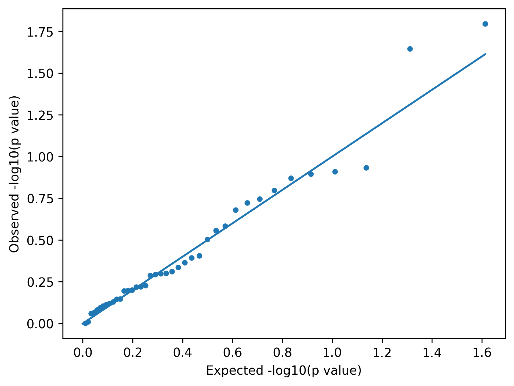
6.8 Key takeaways
- Association testing fits a model per variant
- Covariates help reduce confounding
- QQ plots provide a global diagnostic of p value calibration
Continue to → Lesson 07: Interpreting GWAS Results